Gaussian Process in Action

Building a Gaussian process model with GPyTorch

Gaussian processes (GPs) are a powerful yet often underappreciated model in machine learning. As a non-parametric and Bayesian approach, GPs are particularly effective for supervised learning tasks such as regression and classification. Compared to other models, GPs offer several practical advantages:

• They perform well even with small datasets.
• They provide uncertainty quantification for predictions.

In this tutorial, we will implement GP regression using GPyTorch, a GP library built on PyTorch that is designed for creating scalable and flexible GP models. To learn more about GPyTorch, I recommend visiting their official website.

Note: If you want to follow along with this tutorial, you can find the notebook here.

Setup

Before we begin, we need to install the gpytorch library. You can do this using either pip or conda with the following commands:

pip install gpytorch # using pip
conda install gpytorch -c gpytorch # using conda

Generating the data

Next, we will generate training data for our model by modeling the following function:

\[y = \sin{(2\pi x)} + \epsilon, \epsilon \sim \mathcal{N}(0,0.04)\]

We will evaluate this function at 15 equally spaced points in the interval \([0,1]\). The generated training data is illustrated in the following plot:

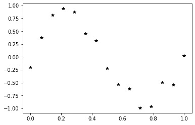
Figure 1. The generated training data by evaluating the true function on 15 equally-spaced points from \([0,1]\).

Building the model

Now that we have our training data, we can start building our GP model. GPyTorch provides a flexible framework for constructing GP models, similar to building neural networks in standard PyTorch. For most GP regression models, you will need to create the following components:

• A GP model: For exact (non-variational) GP models, use gpytorch.models.ExactGP.
• A likelihood function: For GP regression, we typically use gpytorch.likelihoods.GaussianLikelihood.
• A mean function: This serves as the prior mean of the GP. If you’re unsure which mean function to use, gpytorch.means.ConstantMean is a good starting point.
• A kernel function: This defines the prior covariance of the GP. For this tutorial, we will use the spectral mixture (SM) kernel (gpytorch.kernels.SpectralMixtureKernel).
• A multivariate normal distribution: Represented by gpytorch.distributions.MultivariateNormal.

We can build our GP model by assembling these components as follows:

Show code

class SpectralMixtureGP(gpytorch.models.ExactGP):
    def __init__(self, x_train, y_train, likelihood):
        super(SpectralMixtureGP, self).__init__(x_train, y_train, likelihood)
        self.mean = gpytorch.means.ConstantMean() # Construct the mean function
        self.cov = gpytorch.kernels.SpectralMixtureKernel(num_mixtures=4) # Construct the kernel function
        self.cov.initialize_from_data(x_train, y_train) # Initialize the hyperparameters from data

    def forward(self, x):
        # Evaluate the mean and kernel function at x
        mean_x = self.mean(x)
        cov_x = self.cov(x)
        # Return the multivariate normal distribution using the evaluated mean and kernel function
        return gpytorch.distributions.MultivariateNormal(mean_x, cov_x) 

# Initialize the likelihood and model
likelihood = gpytorch.likelihoods.GaussianLikelihood()
model = SpectralMixtureGP(x_train, y_train, likelihood)

Here’s a breakdown of the code:

• The GP model consists of two main components: the __init__ and forward methods.
• The __init__ method initializes the model with training data and a likelihood, constructing necessary objects like the mean and kernel functions.
• The forward method takes the input data x and returns a multivariate normal distribution based on the evaluated mean and covariance.
• We initialize the likelihood function for the GP model using the Gaussian likelihood, which assumes a homoskedastic noise model (i.e., uniform noise across inputs).

Training the model

With the model built, we can now train it to find the optimal hyperparameters. Training a GP model in GPyTorch is akin to training a neural network in standard PyTorch. The training loop involves the following steps:

• Setting all parameter gradients to zero.
• Calling the model to compute the loss.
• Backpropagating the loss to compute gradients.
• Taking a step with the optimizer.

Remark: By creating a custom training loop, we gain greater flexibility in training, such as saving parameters at each step or using different learning rates for different parameters.

Here’s the code for the training loop:

Show code

# Put the model into training mode
model.train()
likelihood.train()

# Use the Adam optimizer, with learning rate set to 0.1
optimizer = torch.optim.Adam(model.parameters(), lr=0.1)

# Use the negative marginal log-likelihood as the loss function
mll = gpytorch.mlls.ExactMarginalLogLikelihood(likelihood, model)

# Set the number of training iterations
n_iter = 50

for i in range(n_iter):
    # Set the gradients from previous iteration to zero
    optimizer.zero_grad()
    # Output from model
    output = model(x_train)
    # Compute loss and backprop gradients
    loss = -mll(output, y_train)
    loss.backward()
    print('Iter %d/%d - Loss: %.3f' % (i + 1, n_iter, loss.item()))
    optimizer.step()

In this code, we first set our model to training mode. Then, we define the loss function and optimizer to use during training. We use the negative marginal log-likelihood as the loss and Adam as the optimizer, running the loop for 50 iterations.

Making predictions

Finally, we can make predictions with the trained model. The routine for evaluating the model and generating predictions is as follows:

Show code

# The test data is 50 equally-spaced points from [0,5]
x_test = torch.linspace(0, 5, 50)

# Put the model into evaluation mode
model.eval()
likelihood.eval()

# The gpytorch.settings.fast_pred_var flag activates LOVE (for fast variances)
# See https://arxiv.org/abs/1803.06058
with torch.no_grad(), gpytorch.settings.fast_pred_var():
    # Obtain the predictive mean and covariance matrix
    f_preds = model(x_test)
    f_mean = f_preds.mean
    f_cov = f_preds.covariance_matrix

    # Make predictions by feeding model through likelihood
    observed_pred = likelihood(model(x_test))

    # Initialize plot
    f, ax = plt.subplots(1, 1, figsize=(8, 6))
    # Get upper and lower confidence bounds
    lower, upper = observed_pred.confidence_region()
    # Plot training data as black stars
    ax.plot(x_train.numpy(), y_train.numpy(), 'k*')
    # Plot predictive means as blue line
    ax.plot(x_test.numpy(), observed_pred.mean.numpy(), 'b')
    # Shade between the lower and upper confidence bounds
    ax.fill_between(x_test.numpy(), lower.numpy(), upper.numpy(), alpha=0.5)
    ax.set_ylim([-3, 3])
    ax.legend(['Observed Data', 'Mean', 'Confidence'])
    plt.show()

The above code performs several things:

• It generates test data using 50 equally spaced points from \([0, 5]\).
• The model is set to evaluation mode, and we utilize gpytorch.settings.fast_pred_var() for faster predictive distributions.
• The trained GP model returns a MultivariateNormal distribution containing the posterior mean and covariance, from which we extract the predictive mean and covariance matrix.
• Finally, we plot the mean and confidence region of the fitted GP model. The confidence_region() method provides the upper and lower bounds, representing two standard deviations above and below the mean.

The resulting plot is shown below:

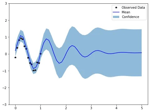
Figure 2. Plot of the fitted GP model given by the mean (blue line) and confidence region (shaded area). The observed data (black stars) is also plotted in the figure.

In this plot, the black stars (★) represent the training (observed) data, while the blue line and shaded area (🟦) indicate the mean and confidence bounds, respectively. Notice how the uncertainty decreases near the observed points. If we added more data points, we would see the mean function adjust to pass through them, further reducing uncertainty close to the observations.

Takeaways

In this tutorial, we learned how to build a GP model using GPyTorch. There are many additional features in GPyTorch that I did not cover here. I hope this tutorial serves as a solid foundation for you to explore GPyTorch and Gaussian processes further.