
Motivation
As an international student studying in China, I’ve always been fascinated by the diversity of Chinese culture and history. This motivated me to build a Chinese calligraphy classifier.
There are multiple styles of calligraphy, which mainly belong to different dynasties. Each of them has its way of shaping and arranging the character. For this project, I picked four styles:
- Seal Script (篆書 zhuanshu)
- Cursive Script (草書 caoshu)
- Clerical Script (隸書 lishu)
- Standard Script (楷書 kaishu)

If you’re interested, you can read more about these different styles here.
Collecting the data
To build a calligraphy classifier, we’re going to need some examples of each style.
However, I did some online search and could not find a decently made dataset for various calligraphy styles.
So, I decided to create the dataset myself.
Fortunately, creating my own dataset isn’t that hard, thanks to Google Images’ search functionality and some JavaScript snippets.
Here’s how I did it:
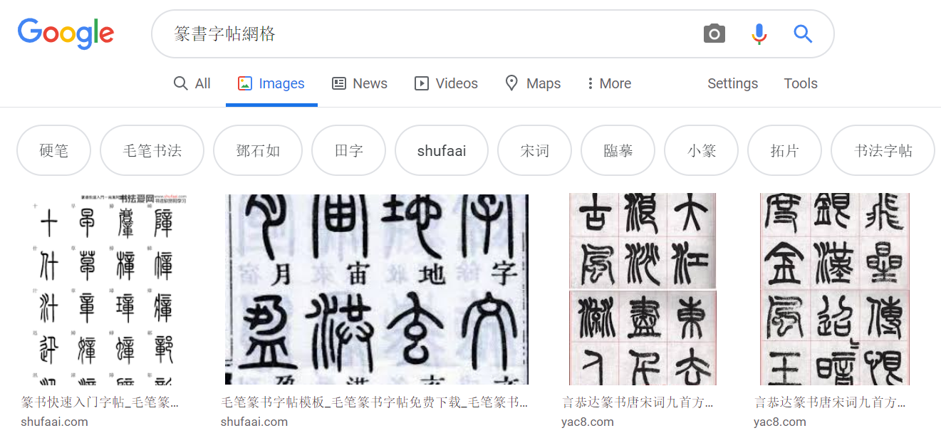
- I searched the images on Google Images and used this keyword format (style + “字帖網格") to get the most relevant results.
- I used this JavaScript code to retrieve the URLs of each of the images.
- I downloaded the images using fast.ai’s download_images function
- Alternatively, I tried using this snippet to automatically download the images from Baidu Images.
Preprocessing the data
After importing the data, I split the data into training and validation set with an 80:20 ratio. The images are also resized to 224 pixels, which is usually a good value for image recognition tasks. Here’s some of the images in the dataset:

Observation: The dataset is rather ‘dirty’. Some of the images are not well-aligned and not properly cropped.
Building the model
For the model, I use the ResNet-50
model architecture with the pre-trained weights on the ImageNet dataset.
To train the layers, I use the fit_one_cycle method based on the ‘1 Cycle Policy’,
which basically changes the learning rate over time to achieve better results.
learn.fit_one_cycle(3)
| epoch | train_loss | valid_loss | accuracy |
|---|---|---|---|
| 0 | 1.469915 | 0.927739 | 0.737500 |
| 1 | 1.075304 | 0.637498 | 0.790000 |
| 2 | 0.820588 | 0.574865 | 0.822500 |
After 3 epochs of fit_one_cycle, I managed to achieve an accuracy of 82% on the validation set.
Tuning the model
By default, the model’s initial layers are frozen to prevent modifying the pre-trained weights. I tried unfreezing all the layers and train the model again for another 2 epochs. To find the perfect learning rate, I used the lr_find and recorder.plot methods to create the learning rate plot.

The red dot on the graph indicates the point where the gradient is the steepest. I used that point as the first guess for the learning rate and train the model for another 2 epochs.
min_grad_lr = learn.recorder.min_grad_lr
learn.fit_one_cycle(2, min_grad_lr)
| epoch | train_loss | valid_loss | accuracy |
|---|---|---|---|
| 0 | 0.484713 | 0.273136 | 0.885609 |
| 1 | 0.491012 | 0.287252 | 0.878229 |
Cleaning the data
fast.ai also provides a nice functionality for cleaning your data using Jupyter widgets.
The ImageCleaner class displays images for re-labeling or deletion.
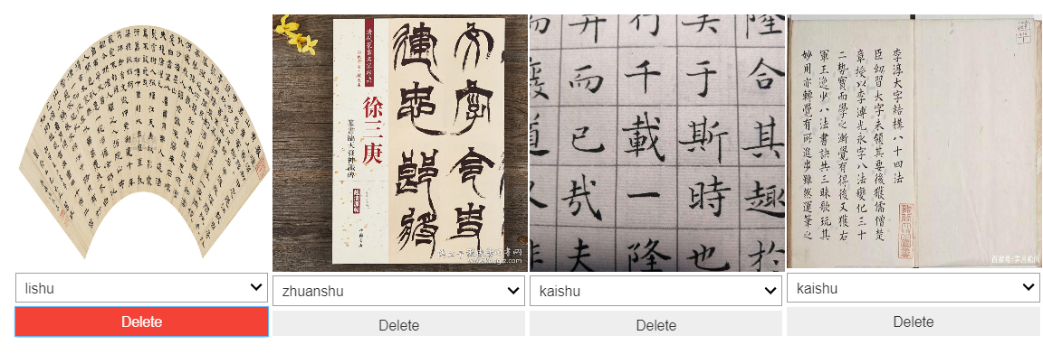
The results of the cleaning are saved as a CSV file which I then used to load the data. I applied the same training steps as above but using the cleaned data.
min_grad_lr = learn.recorder.min_grad_lr
learn.fit_one_cycle(4, min_grad_lr)
| epoch | train_loss | valid_loss | accuracy |
|---|---|---|---|
| 0 | 0.428563 | 0.235304 | 0.922509 |
| 1 | 0.398285 | 0.289792 | 0.892989 |
| 2 | 0.422449 | 0.230904 | 0.926199 |
| 3 | 0.436341 | 0.261377 | 0.915129 |
With only very few lines of code and very minimum efforts for data collection, I managed to achieve an accuracy of 92%. I believe with more and better-quality data, I can achieve a state-of-the-art result.
Interpreting the results
I used fast.ai’s ClassificationInterpretation class to interpret the results.
In particular, I plot the confusion matrix to see where the model seems to be 'confused'.
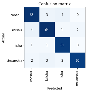
From the confusion matrix, it can be seen that the model does pretty well in classifying the 'zhuanshu' style.
This is probably due to its unique stroke arrangements.
To wrap up, I also plotted the ground truth vs. predictions by calling the learn.show_results method.
